
2017 Eclipse Experiment Description
Experiment Summary
Scientific Questions
- How much of the ionosphere is affected by a solar eclipse?
- For how long is the ionosphere affected by a solar eclipse?
- What causes these spatial and temporal scales?
Methodology
- Illuminate the ionosphere with an Eclipse QSO Party.
- Use networks such as the Reverse Beacon Network to collect data.
- Use amateur radio data to complement data from other sources.
Introduction
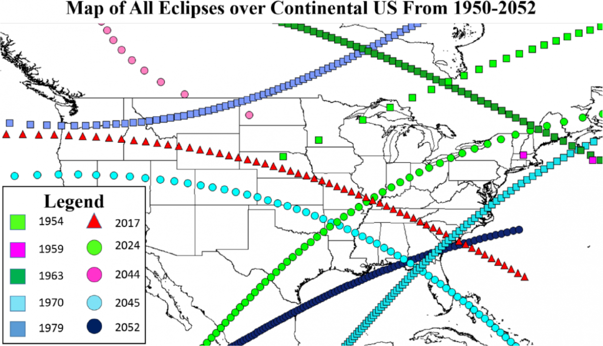
On 21 August 2017, a total solar eclipse will cause the shadow of the moon to traverse the United States from Oregon to South Carolina in just over 90 minutes. As shown in Figure 1, this will be the one of most significant solar eclipses traversing the continental United States for 100 years. While solar eclipses are perhaps best known for their stunning visual display, the shadow of an eclipse also causes changes to the ionosphere which effect radio wave propagation and are useful for the study of ionospheric physics. For a summary of ionspheric radio effects as measured during the 1999 United Kingdom Total Solar Eclipse, please see Bamford 2000.
Although the ionospheric effects of solar eclipses have been studied for over 50 years, many unanswered questions remain. Some include, “How much of the ionosphere is affected by the solar eclipse, and for how long? Why is this the case?” HamSCI is inviting amateur radio operators to participate in a large-scale experiment which will characterize the ionospheric response to the 21 August 2017 total solar eclipse and target these open questions in ionospheric physics.
|
Figure 1: Total solar eclipses visible in the US from 1950 to 2052. The 2017 eclipse (red triangles) will have an exceptionally long footprint in the heart of the continental US. |
Background
The ionosphere is produced when solar ultra violet (UV) and x-ray radiation cause neutral atoms and molecules in the Earth’s atmosphere to be stripped of negative electrons. This creates a type of gas known as a plasma, which is made of both positively and negatively charged particles. After a certain amount of time, some of these particles recombine to form neutrals again. When solar radiation is present, ionospheric production and loss processes occur simultaneously creating a strong ionosphere. When solar radiation is absent, loss processes dominate and the ionosphere becomes weaker. These effects are most commonly observed as a result of the day-night (diurnal) cycle. Figure 2 shows examples of typical day and night ionospheric profiles generated using the International Reference Ionosphere (IRI) empirical model [Bilitza et al., 2011].
|
Figure 2: Typical day (red) and night (blue) ionospheric profiles. |

In some ways, the shadow of a solar eclipse is similar to the darkness of night. However, there are significant differences between solar eclipses and typical day-night variations. For instance, an eclipse shadow moves faster than and in the opposite direction of the dusk or dawn terminators. Additionally, an eclipse shadow is relatively localized compared to night. Because the ionosphere does not respond instantaneously to changes in solar inputs, and several processes in addition to simple ion production and recombination are at play, it is not possible to assume that the ionosphere will respond to an eclipse in the same manner as dusk or dawn.
Previous solar eclipse studies have found that ionospheric densities at lower altitudes (D and E regions, 60 – 150 km altitude) deplete rather quickly. Conflicting results have been reported for the F region (150 – 600 km altitude), which is a region that is more effected by plasma transport processes than photoionization. Typically, it has been reported that these conditions allow for better radio wave propagation at lower frequencies (< 10 MHz) during the eclipse, as D and E region absorption disappears during this time.
Scientific Merit
Important open questions refer to the spatial and temporal scales of eclipse ionospheric effects. Eclipse totality affects only a narrow region of the Earth’s atmosphere (on the order of a few hundred kilometers) for time periods of less than ten minutes. However, previous observations suggest that ionospheric effects are much larger and longer than might be expected. Figure 3 and Figure 4 illustrate this. Figure 3 shows the F2 region peak critical frequency (foF2) over Chilton, England during a total solar eclipse on 11 August 1999. The green line shows measurements made with an ionosonde [Afraimovich et al., 2002], while the blue line shows the expected (non-eclipsed) values generated by the IRI. The measured values depart from the expected values from 0800 to 1200 local time, much longer than the less than 10 minutes of totality.
|
Figure 3: Effect of the August 11, 1999 eclipse on foF2. The decrease in the observed foF2 (green) from the IRI model (blue) over a long period coincides with partial obscuration of the solar disk. |

Similarly, Figure 4 shows 130.4 nm UV airglow data measured by the Special Sensor Ultraviolet Spectrographic Imager (SSUSI) satellite instrument on days before (left), during (middle), and after (right) a total solar eclipse over Africa on 29 March 2006. The middle panel shows a blue line indicating the totality path, as well as a large region (~3300 km diameter) of depleted airglow that roughly corresponds with the region of partial eclipse shadow. Recent studies, such as [Choudhary et al., 2011], suggest that complex plasma processes may cause larger spatial regions of the ionosphere to be affected than would be predicted by simple photochemistry.
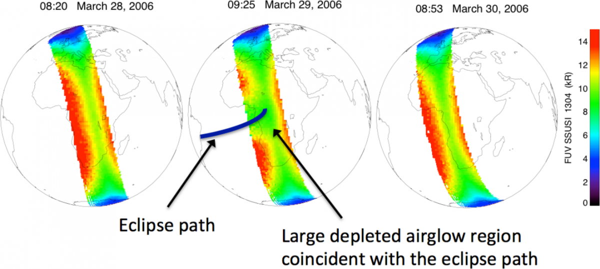 Figure 4: Special Sensor Ultraviolet Spectrographic Imager (SSUSI) airglow data showing a large depleted airglow region associated with a total eclipse in 2006. The three panels show data from days before, during, and after the eclipse at roughly the same location and local time. Figure 4: Special Sensor Ultraviolet Spectrographic Imager (SSUSI) airglow data showing a large depleted airglow region associated with a total eclipse in 2006. The three panels show data from days before, during, and after the eclipse at roughly the same location and local time. |
Although the ionospheric effects of total solar eclipses have been studied for over 50 years, these questions regarding the spatial and temporal scales of eclipse effects have not been adequately answered. There are a number of reasons for this. First, eclipses are relatively rare events which do not frequently traverse geographic areas which are well instrumented for ionospheric studies. Next, technological advances have made it only recently possible to monitor the ionosphere over very large geographic areas with both high temporal and spatial resolution. Finally, the ionospheric response to an eclipse is dependent on season, time of day, and location on Earth (due to differences in the shape and orientation of the Earth’s magnetic field at different locations). This makes every eclipse uniquely valuable for scientific study. The 21 August 2017 eclipse will take place over a large geographic region which is well instrumented for studying ionospheric effects, and therefore presents an excellent opportunity for characterizing the spatial and temporal aspects of the ionospheric response.
Amateur Radio as a Scientific Instrument
Amateur radio operators routinely use frequencies spread across the medium and high frequency bands (1.8 – 30 MHz) to engage in two-way communications across large geographic areas. Details of these communications are recorded in private logs, as well as a public computer network known as the DX Cluster. Recent advances in information technology, signal processing, and software defined radio (SDR) have led to the development of automated observation and reporting systems such as the Reverse Beacon Network (RBN). It has been shown that data from these systems can be used to identify and characterize large-scale ionospheric disturbances [Frissell et al., 2014].
Figure 5 and Figure 6 illustrate diurnal propagation effects observed by the RBN. Figure 5 shows a 5 min interval when both the United States and Europe are in darkness, while Figure 6 shows a 5 min interval when both continents are in daylight. RBN traffic is indicated by lines color-coded by frequency. Black dots indicate RBN receiving stations. Colored dots represent GPS-TEC measurements, which are discussed in the next section. The RBN data shown in these figures characterizes what is typically expected of day and night HF propagation and ionospheric conditions. That is, nighttime conditions (Figure 5) are dominated by communications on frequencies less than 10 MHz, indicating a weaker ionosphere which reflects lower frequencies but cannot refract higher frequencies. Daytime conditions (Figure 6) are dominated by communications on frequencies greater than 10 MHz, indicating a stronger ionosphere which refracts higher frequencies but absorbs lower ones.
 Figure 5: RBN Network Traffic between the US and Europe during nighttime conditions. Note that the green links represent low frequencies, because absorption is minimal in nighttime conditions. Figure 5: RBN Network Traffic between the US and Europe during nighttime conditions. Note that the green links represent low frequencies, because absorption is minimal in nighttime conditions. |
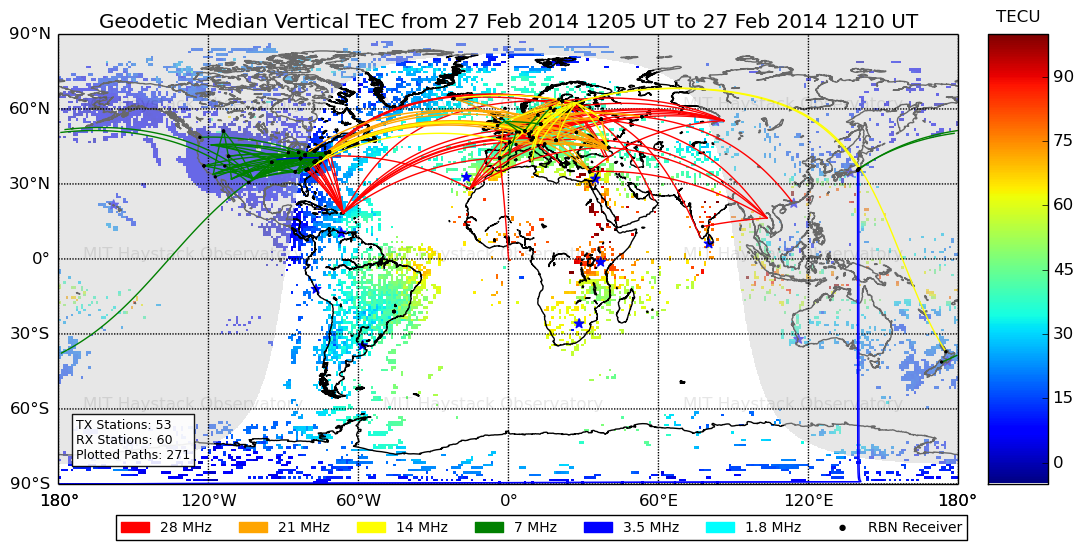 Figure 6: Same format as Figure 5, but for daylight conditions. Note that the red and orange links correspond to higher frequencies, which are less effected by D and E region absorption. Figure 6: Same format as Figure 5, but for daylight conditions. Note that the red and orange links correspond to higher frequencies, which are less effected by D and E region absorption. |
Using this and other similar techniques, HamSCI will use amateur radio data to characterize the spatial and temporal response of the ionosphere to the 21 August 2017 total solar eclipse. It has been recognized that the use of amateur radio signals presents certain challenges for scientific analysis. Some of these challenges include the tendency of operators to transmit only on frequencies which provide the best communication links, a possible lack of amateur radio operations during the period around the eclipse, and an uncertainty as to what equipment (e.g., antenna pattern, transmit power level) is in use. HamSCI intends to mitigate these factors by partnering with the American Radio Relay League (ARRL) to sponsor an Eclipse QSO Party, or contest-style operating event which takes places during the eclipse. The rules of this operating event will be written in such a way to help optimize the experiment. The Radio Society of Great Britain (RSGB) sponsored a similar event during the 20 March 2015 solar eclipse in Europe. Additionally, the operators of the Reverse Beacon Network have joined the HamSCI organization and are working to make improvements to the scientific capabilities of the network.
Additional Ionospheric Instrumentation
In addition to amateur radio observations, many additional, well-established space physics instruments will be used to monitor ionospheric conditions during the 21 August 2017 total solar eclipse. These include measurements by the Super Dual Auroral Radar Network (SuperDARN), Global Positioning System Total Electron Content (GPS-TEC) receivers, ionosondes, and more. Each of these instrument networks sense the ionosphere in a different way and in different locations. Combining the data from these networks together will allow for the most complete characterization of the ionospheric response to the eclipse as possible.
As an example of how this additional data will be used, Figure 5 and Figure 6 show GPS Total Electron Content (GPS-TEC) data beneath the Reverse Beacon Network propagation paths. TEC is a measure of the total number of electrons in the ionosphere on a path between a GPS satellite in space and a GPS receiver on the ground. The speed of a radio signal through the ionosphere is directly related to both the frequency of operation and the density of the ionospheric plasma it travels through. Because certain GPS receivers receive two separate GPS frequencies simultaneously, it is possible to determine the delay between the received signals and estimate the total number of electrons in a column along the propagation path [Rideout and Coster, 2006]. Each TEC Unit (TECU) is equal to 1016 m-2 electrons. Figure 5 and Figure 6 show that, as expected, TEC is high in daytime regions, but low in the night. It is worth noting that due to ground-based receiver requirements, GPS-TEC measurements are only available over and near certain landmasses. There is no coverage over the oceans, and somewhat limited coverage in the middle of the United States. Amateur radio data has the potential to provide information about the ionosphere in places where GPS-TEC data is not available.
Summary
On 21 August 2017, a total solar eclipse will traverse the continental United States from Oregon to South Carolina in a period of just over 90 minutes. Previous research shows that the shadow of the eclipse will impact the ionospheric state, but has not adequately characterized or explained the temporal and spatial extent of the resulting ionospheric effects. HamSCI is inviting the amateur radio community to contribute to a large scale experiment by participating in an Eclipse QSO party and further developing automatic observation networks such as the Reverse Beacon Network. Data resulting from these activities will be combined with observations from existing ionospheric monitoring networks in an effort to characterize and understand the ionospheric temporal and spatial effects caused by a total solar eclipse.
References
Afraimovich, E. L., E. A. Kosogorov, and O. S. Lesyuta (2002), Effects of the August 11, 1999 total solar eclipse as deduced from total electron content measurements at the GPS network, J. Atmos. Solar-Terrestrial Phys., 64(18), 1933–1941, doi:10.1016/S1364-6826(02)00221-3.
Bamford, R. (2000), Solar Eclipse 11 August 1999: Project Final Report, Radio Communication Research Unit, Rutherford Appleton Laboratory, arXiv:1703.01491.
Bilitza, D., L.-A. McKinnell, B. Reinisch, and T. Fuller-Rowell (2011), The international reference ionosphere today and in the future, J. Geod., 85(12), 909–920, doi:10.1007/s00190-010-0427-x.
Choudhary, R. K., J.-P. St. -Maurice, K. M. Ambili, S. Sunda, and B. M. Pathan (2011), The impact of the January 15, 2010, annular solar eclipse on the equatorial and low latitude ionospheric densities, J. Geophys. Res. Sp. Phys., 116(A9), A09309, doi:10.1029/2011JA016504.
Frissell, N. A., E. S. Miller, S. R. Kaeppler, F. Ceglia, D. Pascoe, N. Sinanis, P. Smith, R. Williams, and A. Shovkoplyas (2014), Ionospheric sounding using real-time amateur radio reporting networks, Sp. Weather, 12(12), 651–656, doi:10.1002/2014SW001132.
Rideout, W., and A. Coster (2006), Automated GPS processing for global total electron content data, GPS Solut., 10(3), 219–228, doi:10.1007/s10291-006-0029-5.